Mechanical Measurements and Uncertainties

Índice

1. About Laboratory Teaching
1.1. Measurement Vocabulary
1.1.1. True Value
1.1.2. Measured Value
1.1.3. Measurement Error
1.2. Uncertainty
1.3. Calculation with Uncertainties
1.3.1. Addition
1.3.2. Product
1.3.2.1. Relative Uncertainty
1.3.3. Power
1.3.4. Division
1.3.5. General Expressions
1.3.6. Transcendental Functions
1.3.6.1. Circumventing Maxima/Minima in Sine and Cosine
2. Python Code
3. Flutter Calculator

LabCalc represents a set of tools developed throughout my career as a professor and coordinator of the Physics Laboratory at UVV (Universidade Vila Velha do ES), with the purpose of harmonizing the mathematical methodologies used and enabling a more consistent quantitative assessment of the laboratory works presented by students.

The mathematical theory employed in these tools adopts a simplistic yet effective approach in the manipulation of mechanical measurements and in quantifying experimental uncertainties. Although simplistic, the mathematical approach proves reasonable and effective in laboratory work, albeit with some limitations.

As inherent in any mathematical approach to this subject, it involves a considerable volume of mathematical operations, susceptible to errors, however simple the applied theory may be.

This article presents the mathematical methodology used in these tools, which, despite some limitations and inaccuracies in certain circumstances, stands out for generating quite reasonable results for implementation in higher education and being highly modular.

This modularity facilitates the implementation of this theory in any programming language that supports the object-oriented paradigm and operator overloading, or even through functional programming.

This article aims to present the underlying mathematical foundations of this theory and, in conclusion, I highlight two practical implementations, one in Python 3 and the other a scientific calculator application in Flutter.

About Laboratory Teaching

From 2001 to 2021, I served as the coordinator and technical head of the Physics Laboratory at UVV. Initially, I sought to implement a teaching method strongly based on the reference acquired in the Physics Laboratories of UFES (Federal University of ES), consisting of:

Introducing students to a tool for the development of essential calculations in laboratory work, highlighting the mathematical foundation presented in this article;
Providing material with guidelines for the preparation of reports, emphasizing the evaluation and interpretation of results, as well as graphical analyses;
Supplying scripts with clear objectives and instructions for conducting experiments in the laboratory;
Assessing based on reports that explore the results obtained in the experiments, accompanied by a substantiated analysis.

While the process seems functional in theory, practical complexities emerge. More evident errors in procedures and equipment use can be identified and corrected during the execution of experiments. However, slight variations in equipment setups and the numerous possibilities for errors in the mathematical operations needed to achieve the final results contribute to a considerable dispersion of results.

In the end, this process can become exhaustive for the students, leaving little energy for the final analysis of the results. This sometimes results in vague conclusions and weakly founded on the procedures carried out, or even on the physics of the problem addressed.

It is a fact that it is important for students to understand the mathematical procedures employed in calculating their experimental results, as well as the limitations of the mathematical models used. However, this should not be the ultimate goal.

LabCalc, as conceived, aims to provide a tool that simplifies this part of the work, speeding up the mathematical processes and allowing a greater focus on the analysis and discussion of the results obtained.

The mathematical method adopted here represents a simplification of classic models, without significant losses.

Measurement Vocabulary

Before delving into the mathematical model for calculation with uncertainties, it is crucial to establish a basic nomenclature about measurements and operations in the laboratory. I do not intend to dwell excessively on these aspects.

True Value

The True Value represents the exact measurement of a physical quantity, something that, in general, does not exist. The True Value of a measurement is only achieved in standards, such as a standard for mass, length, or time.

Consider an experiment to measure the length of an object maintained under constant temperature and pressure. When measured with a ruler in centimeters, the value read on the scale might be $12.5\,cm$ . On a ruler in millimeters, the measured value might be $12.45\,cm$ . Using equipment with a precision of 1 micrometer, the measured value can be refined to something like $12.458\,cm$ .

Is it possible to extend this process with even more precise equipment until reaching the True Value of this length?

The answer to this question is no. Even if the object is cut with the best equipment available in current technology, there will come a point where surface imperfections will be detected by the measuring equipment, resulting in different values in subsequent measurements of the same length. This happens due to small imperfections on the surfaces being measured by the equipment.

Generally, this can be observed when trying to measure the diameter of a steel sphere with a micrometer. With each measurement, if the equipment is removed and repositioned, small variations of a few microns will be noted between the different measurements.

Measured Value

Thus, there is no true value for the diameter of a sphere, but rather a Measured Value. This represents the value obtained by the equipment used, considering the specific conditions at the time of its execution.

Unless we are in a Standards of Weights and Measures laboratory, we deal exclusively with Measured Values.

Measurement Error

A mechanical measurement transcends the simple reading of a scale, involving a set of procedures aimed at minimizing procedural or even accidental errors, such as:

Presence of impurities on the surface of the object to be measured or on the equipment’s clamps;
Need for calibration;
Possibility of incorrect positioning of the equipment during measurement;
Occurrence of parallax error, when viewing the scale at a non-right angle;
Impact of mechanical vibrations on the measuring object or scale;
Difficulties or impossibility of adequate positioning of the scale, among other factors.

The discussion on measurement errors is extensive, and I do not intend to delve deeply into this topic, as it is not the focus of this text. However, even under ideal operational conditions, meticulously cleaned surfaces, and highly qualified operators, we still face the previously mentioned limitations.

In a simplified form, these operational errors introduce an inherent imprecision to the measurement, which we will call uncertainty.

Uncertainty

Uncertainty is an attempt to quantify the reliability of the result of a measurement by establishing a validity interval for the measurement. This interval should contain the best possible value for the measured quantity, encompassing both operational errors and the limitations of the equipment, measurement conditions, or imperfections of the measured object.

Methodologies and procedures for determining the appropriate uncertainty in a measurement can vary between different laboratories, depending on their methodologies, equipment, and technical rules. It is not the aim of this text to delve into these particularities, leaving that responsibility to the laboratories to determine their own methodologies.

With this in mind, a length measurement can be expressed, using uncertainty, in the following way:

$\begin{equation*} m_0 = (12.56 \pm 0.03 )\,cm \end{equation}$

This measurement implies that any value between $12.53\,cm$ and $12.59\,cm$ is equally probable for the Measured Value of this length. Thus, the uncertainty expresses the measurement in the form of a range, in this case, $\pm 0.03\,cm$ around the central value, $12.56\,cm$ .

When dealing with uncertainties, it is crucial to understand that the value $12.56\,cm$ is as valid as any other value in the range of $12.53\,cm$ to $12.59\,cm$ , and therefore, does not have preference over any other value within the interval.

Suppose you conduct an experiment to determine the concentration of a particular element in a sample through indirect measurements of other physicochemical properties of the sample. After measuring the properties of the sample and employing a physicochemical model for the problem, in addition to some calculations, you obtain the answer for this experiment as:

$\begin{equation*} c = (11.66 \pm 0.08 )\,\text{Mol/L} \end{equation}$

This means that the concentration of the element in the sample is between $11.58\,\text{Mol/L}$ and $11.74\,\text{Mol/L}$ .

At this point, uncertainty should be seen as a certification that the best Measured Value for this concentration, regardless of the care employed in the measurement or the quality of the equipment used, must necessarily contemplate, at least, a part of the indicated interval.

Otherwise, either some error occurred in the experimental procedure, or the applied model is inadequate for the particular sample or measurement. Obviously, any of these options must be substantiated with solid arguments, and this is essentially what is expected in experimental work.

A more detailed discussion on errors and the determination of uncertainty can be found in metrology courses, where these are meticulously analyzed and treated appropriately.

Calculation with Uncertainties

The following sections address the methodology for performing mathematical operations with measurements and their uncertainties. The model presented is the same introduced in physics laboratory courses at many Brazilian universities, focusing on simplicity and modularity to facilitate implementation in computational tools.

Addition

Let $A$ and $B$ be two measurements:

$\begin{equation*} A = a \pm \Delta a \end{equation}$

$\begin{equation*} B = b \pm \Delta b \end{equation}$

where $a$ and $b$ are the measurements, and $\Delta a$ and $\Delta b$ are their uncertainties. The sum of these two measurements can be calculated as:

$\begin{equation*} A + B & = & (a \pm \Delta a) + (b \pm \Delta b) \\ \end{equation}$

(1) $\begin{equation*} A + B = (a + b) \pm (\Delta a + \Delta b) \end{equation*}$

Therefore, the final uncertainty will be the sum of the uncertainties of the two measurements. Subtraction follows the same process with a slight difference: the uncertainties are always added.

$\begin{equation*} A - B = (a \pm \Delta a) - (b \pm \Delta b) \end{equation}$

(2) $\begin{equation*} A - B = (a - b) \pm (\Delta a + \Delta b) \end{equation*}$

In the end, whether in addition or subtraction, the uncertainties are summed. This expresses that dividing a length to measure it in several stages increases the total length uncertainty, which is reasonable, considering that each measurement has an inherent operational error.

Product

Considering the same measurements $A$ and $B$ presented earlier, we now wish to determine the product $A \cdot B$ . Multiplying the elements term by term, we obtain:

$\begin{eqnarray*} A \cdot B & = & (a \pm \Delta a) \cdot (b \pm \Delta b) \\ & = & a\cdot b \pm (a \cdot \Delta b + b \cdot \Delta a + \Delta a \cdot \Delta b) \end{eqnarray*}$

As $\Delta a$ and $\Delta b$ are generally expected to be significantly smaller than $a$ and $b$ , the last term, $\Delta a \cdot \Delta b$ , is quite small compared to the others and can be neglected, leaving only the first two elements.

$\begin{eqnarray*} A \cdot B & = & a\cdot b \pm (a \cdot \Delta b + b \cdot \Delta a) \\ \end{eqnarray*}$

This equation can also be conveniently written in the form:

(3) $\begin{eqnarray*} A \cdot B & = & a\cdot b \left[ 1 \pm \left( \frac{\Delta a}{a} + \frac{\Delta b}{b}\right) \right] \end{eqnarray*}$

This final form is easier to implement in mathematical operations and also highlights another important element, discussed below.

Relative Uncertainty

This expression introduces a very useful and practical element in the calculation with uncertainties, the Relative Uncertainty. It is defined as the ratio between the Measured Value and its Uncertainty:

(4) $\begin{equation*} IR_A = \frac{\Delta a}{a} \end{equation*}$

That is, the fraction between the uncertainty and the measurement.

Therefore, we can understand the product $A \cdot B$ as being the product times the sum of the relative uncertainties of $A$ and $B$ , as shown below,

$\begin{eqnarray*} A \cdot B & = & a b \pm a b \left( IR_A + IR_B \right) \end{eqnarray*}$

Another interesting use of relative uncertainty is its employment as a precision comparison parameter between two measurements with uncertainties, as the smaller its relative uncertainty, the more precise the measurement. This is illustrated in the numerical example below:

$\begin{eqnarray*} A = 2.25 \pm 0.05 \Rightarrow IR_A & = & 0.05/2.25 = 0.022 = 2.2\% \\ B = 0.012 \pm 0.002 \Rightarrow IR_B & = & 0.002/0.012 = 0.167 = 16.7\% \end{eqnarray*}$

Although the uncertainty of $B$ is much smaller than that of $A$ , the measurement $A$ is more precise than $B$ due to its smaller relative uncertainty.

Power

Now, let’s consider determining the value and uncertainty of the power $A^3$ . In this case, we can do this by applying the product rule to the expression $A \cdot A^2$ , as follows:

$\begin{eqnarray*} A^3 & = & A \cdot A^2 \\ & = & A \cdot \left\{ a a \left[ 1 \pm \left( \frac{\Delta a}{a} + \frac{\Delta a}{a} \right) \right] \right\} \\ & = & A \cdot a^2 \left[ 1 \pm 2 \frac{\Delta a}{a} \right] \\ & = & a \cdot a^2 \left[ 1 \pm \left(\frac{\Delta a}{a} + 2 \frac{\Delta a}{a} \right) \right] \\ & = & a^3 \left[ 1 \pm 3 \frac{\Delta a}{a} \right] \end{eqnarray*}$

In summary, in this expression, we see that the relative uncertainty of $A^2$ is $2 \Delta a/a$ , and of $A^3$ is $3 \Delta a/a$ . By expanding to a power $A^n$ , we can expect its relative uncertainty to be $n \Delta a/a$ . Mathematically extrapolating, we can state that for any $n \in \Re$ , we can expect that:

(5) $\begin{equation*} A^n = 1 \pm |n| \frac{\Delta a}{a} \end{equation*}$

The modulus of $n$ is necessary for negative powers since the uncertainty must always be positive.

Division

At this point, division can be easily determined by employing the relative uncertainty of the power above together with a product:

$\begin{eqnarray*} \frac{A}{B} & = & \frac{a}{b} \left[ 1 \pm \left( IR_A + IR_{B^{-1}} \right) \right] \\ & = & \frac{a}{b} \left[ 1 \pm \left( \frac{\Delta a}{a} + |-1|\frac{\Delta b}{b} \right) \right] \end{eqnarray*}$

which means

(6) $\begin{equation*} \frac{A}{B} = \frac{a}{b} \left[ 1 \pm \left( \frac{\Delta a}{a} + \frac{\Delta b}{b} \right) \right] \end{equation*}$

General Expressions

As observed, the calculation of uncertainty in an operation involving products, divisions, and powers boils down to performing the operation and determining its uncertainty as the result of the operation times the sum of the relative uncertainties. Thus, the product $\sqrt{A/B^5} \cdot C^3$ , where $A$ , $B$ , and $C$ are measurements with their respective uncertainties, can be determined as:

(7) $\begin{equation*} \sqrt{\frac{A}{B^5}}\cdot C^3 = \sqrt{\frac{a}{b^5}} \cdot c^3\left[1 \pm \left(\frac{1}{2}\frac{\Delta a}{a} + \frac{5}{2}\frac{\Delta b}{b} + 3\frac{\Delta c}{c} \right) \right] \end{equation*}$

Transcendental Functions

For functions that cannot be represented by polynomials, the proposed approach here is to use the average of the function’s values at the extremes of the argument as the value and half of the variation as the uncertainty. In other words, if $X = x \pm \Delta x$ represents a value with its uncertainty, the following expressions represent the value of a function $f(x)$ applied to $X$ :

(8) $\begin{equation*} f(X) = \frac{f(x+\Delta x) + f(x - \Delta x)}{2} \end{equation*}$

and its uncertainty,

(9) $\begin{equation*} \Delta f(X) = \frac{|f(x+\Delta x) - f(x - \Delta x)|}{2} \end{equation*}$

The problem with this solution arises when the measurement $X = x \pm \Delta x$ involves a point of maximum or minimum of the function $f(x)$ . One way to circumvent this is to evaluate the function at its maximum/minimum and use this value as one of the extremes for the function.

In a modular application as proposed in this article, the only functions that could generate this problem would be the sine and cosine functions around a point of maximum or minimum.

Circumventing Maxima/Minima in Sine and Cosine

In this case, imagine you want to determine $f(X)$ of a measurement $X = x \pm \Delta x$ where this interval involves a maximum or minimum of the function. Initially, it is necessary to determine if there is a maximum or minimum in the interval. This can be easily verified by observing the derivatives of the functions at $x - \Delta x$ and $x + \Delta x$ .

If there is no maximum or minimum in the interval, it is expected that the derivatives of the function at the extremes of the interval will both be increasing or both decreasing, making the product of these derivatives always positive. However, if there is a maximum or minimum in the interval, the product of the derivatives at both extremes of the interval will always be negative, since before a maximum, the function is increasing, and after the maximum, the function is decreasing, and the opposite occurs in the case of a minimum in the interval.

For illustration, consider the function of the graph below, where $x \pm \Delta x$ involves a maximum. The green and red lines in the following graph illustrate the derivatives of the function at the beginning and end of the interval, indicating a maximum in the interval.

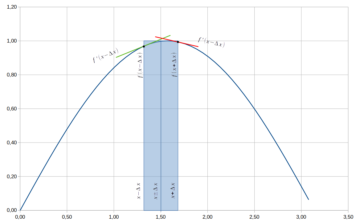
Next, determine which value of $f(x-\Delta x)$ or $f(x+\Delta x)$ is furthest from the maximum. In the above graph, $f(x-\Delta x)$ is further away. Thus, $f(X)$ will be defined as:

(10) $\begin{equation*} f(X) = \frac{f_{max} + f(x - \Delta x)}{2} \end{equation*}$

and its uncertainty,

(11) $\begin{equation*} f(X) = \frac{|f_{max} - f(x - \Delta x)|}{2} \end{equation*}$

Where $f_{\text{max}}$ is the maximum value of the function in the interval.

Obviously, doing this manually can be quite tedious, but the idea is easily implemented in a computational language.

Python Code

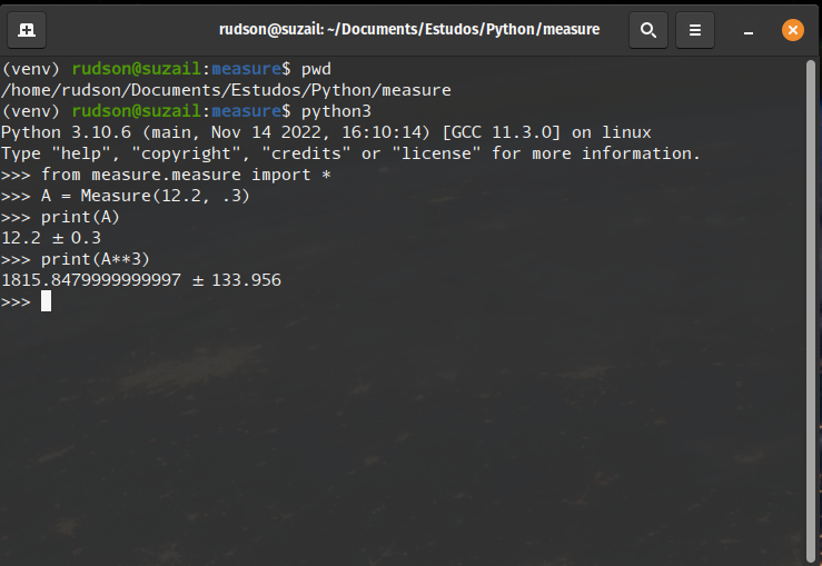
I recently updated a module in Python 3 for Measure, available at github.com/rudsonalves/measure.git. The project is in its early stages but is already functional.

To use it, simply invoke Python 3 and import the Measure module, located at measure/measure.py. Your Python terminal will function as a calculator.

In the future, I plan to implement additional features to the module, such as truncation and more functions.

Flutter Calculator

A preliminary version of the calculator in Flutter is already functional and awaits moderation on Google Play to be made available. I will update here as soon as I have more information.